Statistics is the study of data. The subject’s tools, techniques, and methods allow applicants (statisticians, mathematicians, researchers, etc.) to understand the nature of some data and uncover underlying insights & information within. It is a challenging subject, requires substantial mathematical skills, and compels one to seek reflection paper help from experts.
Yet, mastering stats is all about developing clear concepts and loads of practice. If you are working on a statistics assignment or looking to boost your ideas, this article can help you.
It offers a concise but detailed overview of one of the most effective & commonly used methods in descriptive statistics – measures of central tendency and variability.
What is Central Tendency & What Are The Measures of Central Tendency?
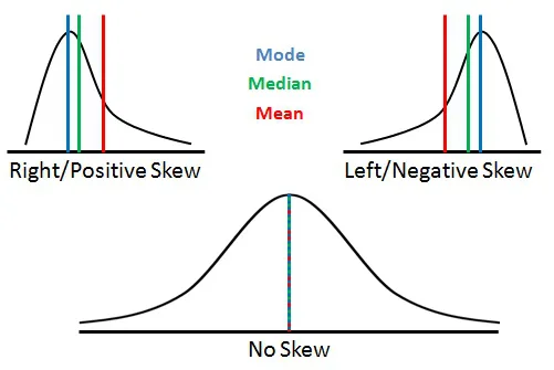
The term central tendency defines typical values of distributions that show how closely the data in a dataset tends towards the center, that is, the concentration of values in the center of the distribution. There are three central tendency measures: mean, mode, and median. All these three measures give us a single value, which defines the general magnitude and characteristics of the data within a set.
All the measures of central tendency in describing & summarizing data provide a variety of functions in data analysis.
- They provide a summary value that can be used to identify the central value or location of the entire data set.
- Vast data sets can be reduced to a single value that acts as an effective representation.
- The mean or average of a sample can be used to determine the population means. Sample means are labeled as statistics, while population means are called parameters.
- Central tendency measures can be used for decision-making.
- Dataset comparisons can be carried out using the measures of central tendency values.
As mentioned, there are three measures of central tendency, each distinct yet related. Let’s have a look.
Mean
Simply put, the mean is the average of all the data in a dataset.
Consider a sample data set, x1, x2, x3, …xn. Then the mean of this sample is denoted by and calculated as follows:
= Σni=1 (xi / n), where n is the number of element s in the set
This is the basic arithmetic mean. There are other kinds, such as geometric mean, weighted mean, and harmonic mean. While we don’t have the time or space to dwell on the other types, here’s a simple article that offers quick insights.
Median
Medians denote the middle value in a set of ordered data. The keyword here is ordered; the data or values in a set must be arranged orderly. The steps to finding the median of a data set involve:
- Arranging all values in an ascending order
- Locating the value by identifying the value at the center of the ordered set
If the number of elements is odd, then median = x(n+1)/2
If the number of elements is even, then median = [Xn/2 + X (n/2) +1] /2, the average of the two values in the expression.
- The value obtained is the median of the ordered dataset.
The above process is applicable for ungrouped data or an individual series. We have a starkly different equation for a continuous series, that is, grouped or class data.
M= l +{[(n/2) – cf]/f * h}
where l is the lower limit of the group in the middle, n is the number of observations, cf is the cumulative frequency, f is the frequency, and h is the class or group size.
Mode
The mode of the dataset is the value that occurs most frequently. One key thing to note is that a dataset can have multiple modes.
If you struggle with sums on measures of central tendency, it is best to seek aid from statistics assignment expert helpers from online custom writing services. Now, let’s look at the measures for determining variability or dispersion.
Measures of Variability or Dispersion
While central tendency depicts the actual value towards which a distribution tends, variability quantifies the degree or extent to which the entries/items/values/elements in a data distribution differ from one another, that is, spread out or clustered together.
Variability allows us to describe distributions and determine how well a sample can be representative of the entire population or distribution. In this article, we will talk about three distinct but related measures of variability, namely, range, interquartile range, and standard deviation & variance.
Range
Range defines the entire scope or spread of a distribution. It is the distance between the largest and smallest elements in a distribution or population. The general process of calculating a range is finding the difference between the upper real limit of the highest value in a distribution and the lowest real limit of the smallest value of a distribution.
Here’s an example for elucidation à
Consider the following distribution – 3, 7, 12, 8, 5, 10
12 is the highest value in this distribution, while 3 is the smallest value. Then, the range of the above distribution will be 12-3= 9.
Again, consider the following class interval distribution – (21-30), (41-50), 61-70), (91-100)
Then, the upper real limit of the highest-class interval is 100, and the lower real limit of the smallest-class interval is 21. The range thus comes around to 100 – 21= 79.
While it is the most obvious measure of variability for distribution, it is considered crude and quite an unreliable measure of variability. The interquartile range is a much more effective measure of dispersion.
Interquartile Range
Ranges are heavily affected by extreme scores in a distribution. The interquartile range measures the scope of the middle 50% of a dataset, bypassing the effects of the extremities. It can estimate the variability where the bulk of the values in a distribution is.
The formula for finding the interquartile range is
IQR = Q3 – Q1
Q3 is the upper quartile of the distribution above which lies the upper 25% of the distribution, and Q1 is the lower quartile below which lies the lower 25%.
To calculate the upper and lower quartile, we first need to find the distribution median. The median divides the entire distribution into two halves. The difference between the upper and lower quartiles gives us the interquartile range. In most cases, we transform the interquartile range into the semi-interquartile range for getting more accurate measures.
The formula for calculating the semi-quartile range is
Semi IQR= (Q3 – Q1)/2
Can you find the IQR and Semi-IQR of the following distribution – 1,2,5,6,9,12,88,96,27,4,34
If you find the above sum or any problem on central tendency & variability measures quite challenging, then statistics assignment help online may become essential.
Standard Deviation & Variance
Considered the most [potent and important measure of variability or dispersion, standard deviation uses the mean of data distribution as the reference point and determines the variability of each element in a distribution from the mean.
Simply put, standard deviation and its counterpart variance show how clustered together or scattered a distribution are. The higher the standard deviation, the more spread out the values are from the mean.
Following are the steps for finding the standard distribution and variance.
- Find the mean of data distribution.
- Find the difference between the mean and every element in a distribution.
- Square the differences or deviations.
- Sum all the squares.
- Divide the sum b (n-1), where n is the number of elements in the distribution, to get the
- Take the square root of the variance to get the standard deviation.
The general formula for finding the standard deviation of any distribution is
Here’s an example
Consider the following distribution: 92, 95, 80, 47, 75, 55
We first need to find the mean of the above distribution, which comes to around 74.
Next, we find the difference or deviation of every element.
| Element | Element- Mean | Difference |
| 92 | 92-74 | +18 |
| 95 | 95-74 | +21 |
| 80 | 80-74 | +6 |
| 47 | 47-74 | -27 |
| 75 | 75-74 | +1 |
| 55 | 55-74 | -19 |
Next up, we need to find the squares of the differences, which come around to à 324, 441, 36, 729,1,361.
The mean of the sum of squares gives us the variance, which here is 315.34
And the square root of the variance gives the standard deviation.
Well, that’s about it for this write-up. Hope it refreshed your ideas about the measures of central tendency and variability. Practice as often as possible and seek professional statistics assignment help online from reputed statistics assignment experts to further boost your ideas & grades.
Author-Bio: Ned Arthurs is a mathematics professor from a major public university in Houston, Texas. He is also a part-time writer and a statistics assignment expert & helper at AllEssayWriter.com. USA’s largest academic service provider.